E-learning in analysis of genomic and proteomic data 2. Data analysis 2.2. Analysis of high-density genomic data 2.2.1. DNA microarrays 2.2.1.7. Analysis of expression arrays

The reason why to search for the differentially expressed genes was motivated in previous chapters. We know already that this is a class comparison problem. The standard methods for calculation of effect sizes, hypothesis testing and regression applied in class comparison were defined in chapter 2.2.1.2. Class comparison. We remind  that the main difference between the two approaches is that the hypothesis testing is an univariate analysis, while regression methods are multivariate. Often, the expression of a gene/protein is affected not only by the group variable, but also by some other variables. The effect of gender or age can serve as simple examples. Older patients have more aberrations than younger patients; genes on X chromosome will be over-expressed in women in comparison to men. Consequently, if we know about the existence of such a factor, we have to account for this effect in the analysis. Regression methods should be used in this case.

There are some other hypothesis testing and regression methods that were desiged especially for expression microarrays. However, these methods can be succesfully applied on all other similar problems such as revealing different abundance of proteins between groups (data from MASS spectrometry, 2D gel electrophoresis, etc...).

In the following we will describe the two additional methods or class comparison: SAM and LIMMA.

 

Significance Analysis of Microarrays (SAM)

Significance analysis of Microarrays (SAM) is a method nowadays widely used for determining changes in gene expression. The method is based on adjusted ordinary t-statistics described earlier.

Let’s have the matrix of gene expression values for n samples and p genes: x_ij, i=1...p and j=1..n, where columns represent samples and rows represent genes, and the group variable y_j, j=1..n, which split samples into two groups, e.g. cancer and normal tissue. Suppose, that we have two groups, then the adjusted t statistics used in SAM is defined as

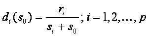
where , p_i and q_i correspond to gene expression means in each group, is common standard deviation for both groups and s₀ is the exchangeability factor, which has to be estimated and makes the difference between t-statistics and SAM. Consequently, if s₀=0, d is an ordinary t statistics, very large values of s₀ make d equivalent to the t-statistic without the nominator. The aim is to estimate s₀ such that the dependence of d on s_i is as small as possible. For the method of s₀ estimation see e.g. Tusher et al. 2001.

Now when the SAM statistics is calculated, we have to set the critical value for significance. Because SAM statistics is no longer an ordinary t-statistics, we can’t use the usual approach of quantiles of t-distribution. Therefore the significance is assessed via permutation procedure suggested in Tusher et.al. (2001).

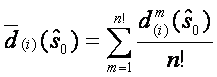
First of all the SAM statistics for all genes are sorted in increasing order: . The next step is permuting the columns of data matrix and assigning first n₁ (number of samples in group one) samples to group 1 and the rest n₂ (number of samples in second group) samples to group 2. A total n!=(n1+n2)!  such permutations are performed. For each permutation the SAM statistics is recorded together with the ordering. The expected order of statistics under the null hypothesis of no difference can be estimated by

Each gene i with its SAM statistics d_i(s₀) considerably larger then  is considered as differentially expressed. Let's denote this distance delta. It is usual to illustrate this by plotting versus expected versus observed calues of SAM:

 

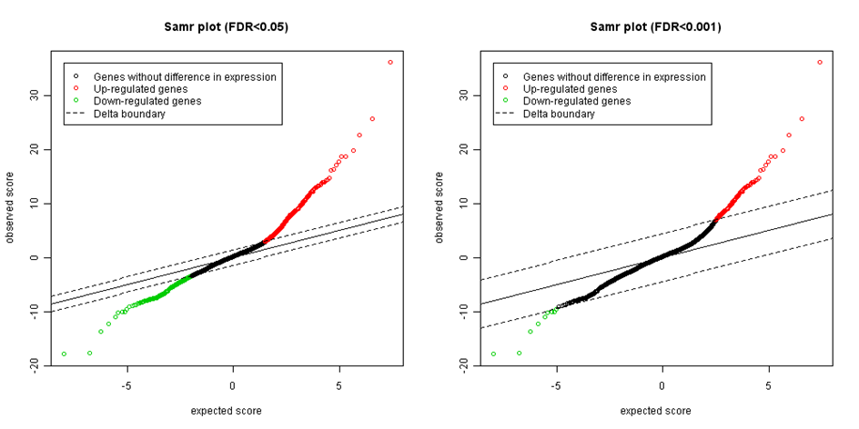
Figure: Expected versus observed SAM statistics with different significance thresholds.

The end tails on both sides represent possible significant genes. The more the points are far from the identity line (the black diagonal), the more likely they are differentially expressed. The last step is setting the appropriate delta . We start with delta=0 and stepwise increase the threshold while controlling the level of false discovery rate (FDR). FDR is computed as median or 90th percentile of the number of falsely called genes divided by the number of genes called significant. There are several strategies, how to select suitable value for delta. For example settle median FDR as high as researcher is willing to tolerate (e.g. 5% or 1%) and then select the smallest value of delta corresponding for such FDR.
After the delta selection, the list of significant genes is returned. However, to filter the genes with no biological effect, the fold change should be calculated.

 

The original documentation to SAM can be downloaded here:

Original documentation

The original paper can be downloaded here:

Significance analysis of microarrays applied to the ionizing radiation response.

For more information, please, consult the SAM webpages:

http://www-stat.stanford.edu/~tibs/SAM/

 

LInear Models for Microrray Analysis (LIMMA)

LIMMA is a package of methods for differential expression analysis in microarrays, based on linear regression. It fits a linear model for each gene separately and uses Empirical Bayesian methods to provide stable results in case of small sample size. The package is implemented in R and provides wide range of functions for both normalization and differential expression data analysis. The linear model and differential expression functions apply to all microarray types, however the normalization functions are available only for two-colour spotted microarrays.

Using limma for differential gene expression analysis

Limma allows defining a wide range of linear models. The basic function fitting the linear model is lmFit. The function requires two entries: a data matrix with rows representing gene expression profiles and columns representing samples and a design matrix.
Design matrix provides a representation of the model we would like to fit, based on explanatory variables to be included. In the following, we will provide some examples of how to set the design matrix appropriately. It has as many rows as number of samples in the experiment. The number of columns differs depending on model design, for example, whether we use intercept or not, how many variables we wish to include in the model and their type.

Design matrix

One-variable example
If we plan to simply compare the gene expression between two groups, we need a very simple design matrix with only 2 columns. First column will contain 1 in all rows, respresenting an intercept; the second column will contain information about the group each sample belongs to. The intercept serves as a reference value (baseline) to which you compare all the effects you wish to estimate. Let’s make a simple model to illustrate. In a room, there is 50 men and 50 women. You wish to know, whether men are higher than women. You assume that men are in average taller than women and you build a linear regression model based on sex. The model can be very simply written as
Height =α + β*Sex
Here αis the intercept that represents the reference value (in our case “average height of women”) and &neta; is the coefficient showing, how many centimeters you have to add to average women height if you wish to obtain average height of men. Sex is the group variable and represents the effect of men, thus in the case of women it has value 0 (our intercept represents already the average height of women), in case of men, the value is 1 (to obtain the average height of men, we increase the average height of women by β).
In each model we need to specify, which group will be the reference one, as this will be coded in our design matrix as 0, the second group will be coded as 1. The reference group is usually the one we compare to, for example normal tissue, wild type bacterial strain, or group of patients that responded to specific therapy. In our example we selected women. The design matrix for our example is of size 100 x 2

Intercept Group
1 1 0
2 1 0
... ... ...
49 1 0
50 1 0
51 1 1
52 1 1
... ... ...
99 1 1
100 1 1

Please note that the first column with row numbers does not make a part of the design matrix.

If we have more than two values on the group variable, we have to specify in our design matrix all the possibilities that can happen. For example, we have to compare gene expression between blood samples from three groups of patients: healthy (H), patients with acute myeloid leukaemia (AML) and patients with acute lymphocytic leukaemia (ALL). Because we wish to study differences between all three groups, each of the three groups should be represented in a model by one variable. Naturally, we choose the healthy patients as a reference to which we wish to compare. These values will be thus captured by Intercept, so we can agree that it is represented as 0 in the model group variable. How do we code ALL and AML? We cannot code them 1 and 2, because this would mean that the group AML has twice as large effect on expression values as ALL. We can code only yes/no, this means 0/1. For this purpose we create so called “dummy variables” storing all the combinations in 0/1 manner .  In our example this means to create two more variables, one coding ALL (0-no, 1-yes) and the second coding AML (0-no, 1-yes).

 

The second is the contrast matrix which allows the coefficients defined by the design matrix to be combined into contrasts of interest.
Each contrast corresponds to a comparison of interest between the RNA targets. For very simple experiments the contrast matrix may not need to be specified explicitly.
 

 Read the original documentation on limma  R package here:

Original limma R-package user guide