E-learning in analysis of genomic and proteomic data 2. Data analysis 2.2. Analysis of high-density genomic data 2.2.1. DNA microarrays 2.2.1.11. Pathway Analysis
2.2.1.11.1.Introduction
Though every microarray experiment starts with a biological question the first steps after hybridisation all deal with data analysis and thus are very much of statistical and mathematical nature. Preprocessing of chips can,
depending on what technology is being used, involve various non-standard statistic tools like non-parametric curve fitting, variance stabilizing transformations and a number of robust statistical methods. The subsequent detection of differentially expressed genes relies heavily on statistical hypothesis testing and again uses advanced techniques like empirical Bayesian methods or complex resampling strategies. Though many of these tools have been implemented in user-friendly software, they typically are conducted by a statistician or bioinformatician, who knows how to make best use of these methods. The first results the biological experimenter sees for his experiment, tends to be a "top table" of differentially expressed genes rank with respect to a p-value or some other score.
For illustration purposes we will use a publicly available data set, that was published Lee et al. [2005]. These authors compared adipose tissue between obese and lean Pima Indians, a group of American Indians that is particular prone to obesity. Samples were hybridised on HGu95e-Affymetrix arrays (12639 genes/probe sets) and the experiment is available as GDS1498 on the GEO database (http://www.ncbi.nlm.nih.gov/sites/GDSbrowser?acc= GDS1498). In order to reduce the complexity of the data set we selected the male samples only, i.e. we have 10 obese subjects that we compare against 9 lean subjects. Using the Bioconductor library limma we conducted a moderated t-test to compare the two group. In table 2.2.1.11.1 we see the list of all genes which have a Benjamini-Hochberg-adjusted p-value below 5%. This would be a typical result file given to a biologist as ”the result” of his experiment.
Table 2.2.1.11.1. List of all genes with adjusted p-value below 5%
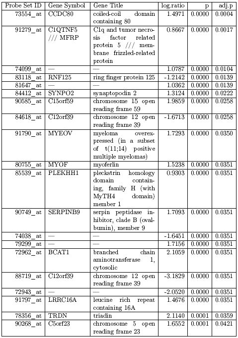
Overall this table consists of 18 genes, some of these the biologist might know about, for others he could use internet resources like gene databases or even Wikipedia to find more about them. For example he might know from the literature that the gene RNF125 is related to immune response. But does that automatically mean that the immune response in the obese subjects is different from the one in lean subjects?
It is this type of question that pathway and gene set analysis is trying to answer. All genes on our array that relate to immune response form, what we call a gene set. And rather than giving a score (e.g. p-value) to single genes like in table 1, we want to give a score to the complete gene set. In this article we will outline some of the basics for this type of analysis. It is not our intention to give a comprehensive overview of all methods; articles by Nam and Kim [2008] and Huang et al. [2009] are good references for that type of review. This text is rather meant as an introduction to the topic for readers that are new to this area.
In Section 2 we will describe how we can identify the genes on our micrarray that belong to a gene set, e.g. that are related to immune response. We will introduce some of the essential internet databases that provide such information and particularly discuss the different types of gene sets that can be used. In Section 3 we study some of the principles in how to test whether a given gene set is significantly differentially expressed. We will not so much discuss the many different methods suggested for this in detail but rather explain some of the most important building blocks of these methods and the different philosophies behind them. We will particularly discuss the difference between self-contained and competitive methods. In Section 4 we will have a look at some selected software tools to perform such gene set analysis and finish the paper with some conclusions in Section 5.