E-learning in analysis of genomic and proteomic data 2. Data analysis 2.3. Analysis of high-density proteomic data 2.3.2. MASS spectrometry 2.3.2.2. Statistical issues in the analysis of proteomic profiles

2.3.2.2.2.1 Pre-processing

Numerous data analytic pre-processing steps must be carried out before statistical models can be applied to MS profiling data:

Calibration
Time-of-flight measured by the spectrometer is converted to the m/z scale using a number of calibrants with known m/z values.

Baseline subtraction
Baseline “noise” is removed from the matrix, for example by locally applied smoothing techniques such as Loess smoothing.

Normalisation
Data are normalised or standardised in some way to create comparability between spectra. The aim of normalization is to remove technical sources of variation (machine performance, sample amount, etc). One commonly-used approach is to standardise by the (local or global) total ion current. Concerns have been raised that this may remove relevant biological information as well as the desired experimental variability (Cairns et al, 2008). Optimal methods of normalization are an area of ongoing research.

2.3.2.2.2.2 Peak alignment and detection

There is imprecision on both the x (m/z) and y (abundance) axes which makes the combining or comparison of profiles complex. Peaks in any one spectrum are local maxima and may be defined as points that are maximal within +/- n points on either side (which we will refer to below as a peak of size n). The signal-to-noise ratio must also be considered, and it is usual to stipulate that peaks must exceed the typical local intensity values by a certain ratio.

Even if peaks can be satisfactorily identified in each individual spectrum, how can peaks be aligned across spectra allowing for variability in x? There are numerous methods of peak detection, none of which is perfect. For example, Morris et al (2005) proposed forming a single spectrum from the mean of all spectra and applying a peak-detection algorithm based on wavelets to this single composite spectrum. This method avoids the issue of peak alignment and is based on the premise that a true peak will stand out against the background noise across multiple spectra, minor misalignment merely resulting in broader peaks. Tibshirani et al (2004) suggested applying a one-dimensional clustering algorithm to the m/z values of peaks across spectra. Tight clusters should represent the same biological peak, possibly shifted slightly along the x-axis. In their method the centroid of each cluster is then used as the consensus m/z value for that peak.

In our Institute we have proposed and applied a method where each spectrum is first smoothed using progressively wider moving averages (Rogers et al, 2003; Barrett and Cairns, 2008). Peaks of size n in each of these smoothed spectra (local maxima with at least n lower points at each side) are identified for successively larger values of n. A frequency distribution is created of the number of times a peak is detected at each point, and from this consensus peaks are determined. To score peaks, each spectrum is then compared to the resulting peak list to determine presence/absence of the peak (within a certain window of tolerance). If the peak is present, then the largest abundance measurement within this window is recorded as the peak abundance for that spectrum. Not all peaks can be detected in each spectrum, and it is a subject of research to consider how to treat “absent” peaks in subsequent analyses (for example as zeroes, missing values or censored below a certain limit).

After all this processing, the data from each initial 2-dimensional spectrum are reduced to a vector of abundance measures for a fixed set of typically several hundred peaks.

The methods outlined below relate to proteomic studies where the analysis is based on peak data and the main aims are to:

•  Identify peaks that differ between two or more groups
• Develop a classification scheme which can be applied to categorise new samples

2.3.2.2.2.3 Multivariate exploratory data analysis

Proteomic profiling data is multivariate, consisting of measurements on numerous inter-correlated peaks. Exploratory data analysis is useful to explore gross differences between groups. One simple such analysis is to visually compare the mean spectra for the two (or more) groups.
Principal components analysis (PCA) can be used to investigate the pattern of variation more fully. PCA is a method of reducing the dimensionality of data based on decomposition of the covariance matrix. The first principal component is the linear combination of variables (peak abundances in this case) that explains the greatest proportion of the overall variance; subsequent components are the orthogonal linear combinations that explain the greatest proportion of the remaining variance.

This is illustrated by applying the method to a study of renal transplantation (unpublished data). Proteomic profiles were obtained using samples from 50 renal transplant recipients (30 with clinically-defined stable condition and 20 with unstable condition), 30 healthy controls and 30 patients with renal failure (prior to dialysis). There was a similar age and gender distribution in each group and an identical protocol for sample handling and processing was used throughout. Samples were randomised to chips and all analysed in duplicate. Three SELDI chip types (H50, IMAC and CM10) were used. By plotting the samples in the 2-dimensional space formed by the first two principal components, we can see how well groups are separated (Figure 2.3.2.4).

 

Figure 2.3.2.4 Scatterplot of first two principal components according to patients stage

It is clear that healthy controls and patients with renal failure form separate clusters, both overlapping with the transplant patients who are somewhat intermediate. A second plot where the analysis is repeated using just the 50 transplant patients (Figure 2.3.2.5) shows that the stable and unstable patients do not appear to be well separated.

Figure 2.3.2.5 Scatterplot of first two principal components according to transplant stable

2.3.2.2.2.4 Statistical methods to detect differences between groups

The first aim to be addressed here is to identify which peaks (if any) differ between two groups (e.g. cases and controls). A simple approach is to carry out a test, such as the two-sample t-test, to compare the groupß means for each peak. To allow for duplicated samples, this can be extended by using a linear random effects model.
For person i, replicate k, the abundance measurement y_ik for a particular peak is modelled by

y_ik = α + ßx_i + η_i + ε_k

where x_i is indicator (1/0) of group (case/control) status, η_i is a random effect term corresponding to subject i and ε_ik represents residual variation, including measurement error. These last two terms are assumed to be normally distributed with mean zero: η_i ~ N(0, σ_u²), ε_ik ~ N(0, σ_e²). A test for a difference between groups is provided by testing whether β is significantly different from zero. This model provides a flexible framework in which covariates can easily be included. In addition an estimate of intra-individual variability is provided by the variance σ_e², which can be compared with the overall variance σ_e² + σ_u². Conversely an estimate of reproducibility is provided by the intra-class correlation coefficient σ_u² / (σ_e² + σ_u²), where values close to 1 indicate good agreement between duplicates.

Sample size calculations

The sample size needed to achieve a particular power to detect differences between groups depends on intra- (σ^₂) and inter- (τ^₂) sample variance, the number (m) of technical replicates and the difference in means to be detected (δ).
For a comparison of two groups, for a particular peak, the number of samples n required in each group is

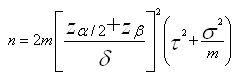
where α is the significance level and 1-β the power (Cairns et al, 2009).
In order to calculate sample size, estimates of variance are therefore needed; sample size requirements depend heavily on the intra-and inter-sample variance of the abundance measures for the peak.
Using pilot data, σ² and τ² can be estimated. However since there are multiple (probably several hundred) peaks to be considered, but only one sample size to be used, the estimates of variance to be used in the calculation could be the median, 90^th percentile or maximum variance across all peaks. Generally using the maximum is too conservative, and the median is unsatisfactory since this implies that power will be lower than desired for 50% of the peaks. A good compromise is therefore the 90^th or 80^th percentile. The estimate of variance used, and hence also which percentile is used in the calculations, has a large impact on the sample size needed for the study. Further details and illustrative examples of sample size calculations can be found in Cairns et al (2009).

Multiple testing

Several hundred peaks will typically be tested in a proteomic profiling study. At the discovery stage, the aim is not to demonstrate a difference between groups with certainty, but to ensure that a high proportion of “significant” or highlighted results are true positives. It is therefore more useful to think of the false discovery rate (FDR, the expected proportion of false positives among those declared significant) than the false positive rate (the expected proportion falsely declared positive among those that are truly null, corresponding to the significance level).
Let P be the total number of peaks and π the proportion of peaks that are truly differentially expressed by a particular amount, then the FDR can be estimated by:

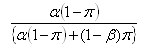
where &aplha; is the significance level and 1-β the power. This relationship can be used to inform the choice of α in order to achieve a particular FDR. Tables illustrating the relationship between the FDR, α, β and π can be found in Cairns et al (2009).

Improving the statistical model

Various improvements have been proposed to the statistical analysis process (e.g. see Hill et al, 2008). For example normalisation and potentially other pre-processing steps could be carried out in the same step as testing and estimating differences between groups in a unified analysis.
In experiments where the identity of proteins and peptides corresponding to the peaks are known, a structure can be imposed on the peaks (peptides within proteins, etc.)

2.3.2.2.2.5 Classification of samples

There are many available classification methods. Here we focus on the Random Forest (RF) classifier (Breiman, 2001).
In a classification tree, variables (peak abundance measures in this context) are used to successively split the sample until all subjects at the same node are in the same class or until a minimum node size is reached. Given a large number of variables compared with the size of the data set, it will generally be possible to perfectly “classify” the samples, but a key issue is to avoid over-fitting the data.
The RF algorithm is a classifier based on a group of classification trees. In each tree, samples are successively split using the variable that “best” discriminates between classes. Usually this is based on the Gini index, a measure of impurity of the nodes. Trees can be grown until each node consists entirely of samples from one class, or alternatively a minimum node size can be set as stopping rule. The idea of RF is to grow many trees and classify on the basis of the majority vote. In order to avoid over-fitting, and to introduce random differences between the trees in the forest, two modifications are made. Firstly, each tree is based on a bootstrap sample of original data set (so that from an initial sample of size m, a bootstrap sample of the same size is obtained by sampling with replacement). Secondly, at each partition only a random subset of the variables is made available to choose from to make the best split. Each tree is used to classify items that are NOT in the bootstrap sample (so called out-of-bag items); a nice feature of the RF algorithm is therefore that it provides an unbiased estimate of classification performance.
 

Breast cancer proteomics data

Several groups met in Leiden in the Netherlands in 2007 to compare methods of classifying samples from breast cancer patients and controls on the basis of proteomics data (Mertens, 2008). The initial data set consisted of MS proteomic profiles from 76 breast cancer cases and 77 controls; profiles from an additional 39 cases and 39 controls were used as validation data. The MS profiles were available after some pre-processing and consisted of abundance measurements for 11,205 points corresponding to m/z ratios along the spectrum.
The analysis described here consisted of a two-stage strategy: peak detection, reducing the 11,205 data points to 365 peaks, followed by application of the RF algorithm to the peak data. Care was taken to minimize dependence on the initial data set of the peak-detection strategy. Details of the method are given in Barrett and Cairns (2008).
Applying RF with 20,000 trees in the forest, and classifying according to majority vote, 84% of the samples were correctly classified. Importantly, when the same classification rule was applied to the independent validation data set, the classification accuracy was very similar (83% correct). In fact, of the methods applied by different groups taking part in the original project, this analysis (using RF applied to peaks) had the joint lowest percentage correct from the initial data, but the highest from the validation data (Figure 2.3.2.6).

Figure 2.3.2.6 Clasiffication: calibration versus validation results

Other methods employed included linear and quadratic discriminant analysis, penalised logistic regression and support vector machines, some of which performed almost as well as RF on the validation data (but overestimated performance on the initial data set). An evaluation of the methods can be found in Hand (2008).