E-learning in analysis of genomic and proteomic data 2. Data analysis 2.1. General analysis workflow 2.1.2. Class comparison (searching for differences between classes) 2.1.2.3. Regression strategies
Regression is a powerful tool, when used appropriately. Regression analysis represents a set of methods which search for the relationship between dependent variable and one or more independent variables. It studies a functional dependence of one variable on the other. The independent variables are called predictor or regressor variables and are denoted as X and the dependent variable is called the response variable and usually denoted as Y. The regression in group comparison can answer different questions (again, we use the example of gene expression analysis):
- “How much the gene expression changes when we change the value of a group variable?”
- “How much the gene expression changes when the value of some other, continuous variable changes?”
- “What is the probability that the sample belongs to a certain group given the expression level of a gene?”
In the first and the second question, the gene expression is the dependent variable (predicted variable, outcome), while the group (or the continuous variable) serves as an independent explanatory variable (predictor). To answer these two questions a linear or non-linear regression is used.
In case 1 the predictor is a binomial or multinomial qualitative variable, in case 2 a relationship between gene expression and some quantitative variable is assessed. Selected examples of predictor variables are listed below:
- Binomial (with two possible values)
- Tumor subtype (AML, ALL)
- Response to therapy (responder, non-responder)
- Bacterial strain (wild type, mutated)
- Multinomial (with more than two possible values)
- Tumor subtype (DLBCL subtypes: RARS, RCMD, RAEB1, RAEB2)
- Tumor best response (CR, PR, SD, PD)
- Bacterial strain (wild type, mutant A, mutant B, ...)
- Quantitative
- Survival times (overall survival, progression free survival,...
- The level of some blood marker (.....)
- Gene expression of another gene
- Age
The third question is answered by logistic regression. On the contrary to linear regression, the gene expression serves a predictor variable and the outcome is the group variable.
For both linear and logistic regression, multiple predictor variables can be combined. For instance, we can be interested in revealing the gene expression differences based on both tumor subtype and the age of the patient. Or given the expression values of several selected genes we would like to know what is the probability a patient has a certain tumor type. The latter is used for building predictors.
In the following we describe the linear and the logistic regression in more detail.
2.1.2.3.1. Linear regression
Linear regression models the relationship between dependent variable Y and one or more independent variables X, such that independent variables depends linearly on Y via unknown parameters that have to be estimated from the data.
In our example the Y represents the vector of gene expressions in all samples and X is a matrix of the values of multiple variables (the group variable and for instance age, tumor subtype, response to theraphy). More precisely, each observation yi (gene expression value in one sample) depends on observations of variables xi_group, xi_age,, xi_subtype,, xi_response via mean of unknown parameters. In general, when considering p independent variables and n samples, the model (the relationship between Y and X) is written as follows:

In our example p=4 (we have four independent variables: group, age, tumor subtype and response to theraphy).
Hence, tjere are n equations (for each observation one), which can be written in vector form:
 ,
,
where Y is vector of dependent variable observations, X is so called design matrix where each column represent one independent variable, β the is vector of unknown parameters called regression coefficients, which we are trying to estimate and ε is the error term or noise and captures the variability of all other factors, which are not involved in the model.
Clearly, the values of parameters β1, β2,..., βp are the same for all the observations (samples).
If we decided to apply to our data this model, we have to check the following main assumptions:
- Linearity of the relationship between dependent and independent variables
- Normality of the error term
- Constant variance of the errors (homoscedasticity)
- Independence of the errors
If the above assumptions are not fulfilled, our results may be wrong and seriously biased. Another very important assumption is that the sample size n has to be larger then the number of independent variables p.
Now we know what is the linear regression model and how to obtain the unbiased results, but we still don’t know how to estimate the unknown parameters β. There are several methods for estimating these parameters, here we will mention the simplest and very common estimation method called the least squares method. This method estimates β such that the value of squared differences between observed and estimted gene expression values is minimal:
 .
.
This is equivalent to solving the following equation
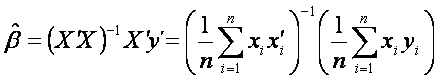 .
.
2.1.2.3.2. Logistic regression
As already mentioned, sometimes we'd rather answer the question "What is the probability that the sample belongs to a certain group given the expression level of a gene?".
In such a situation, when the dependent variable is nominal. or in other words, when we want to predict the probability of occurrence of an event with two possibilities e.g. “disease” or “no-disease”, “male” or “female”, we cannot use the linear regression, because such nominal-scale variable does not follow the normal distribution. Instead, logistic regression can be applied. It may also be extended to cases where the dependent variable has more then two possible categories.
Logistic regression is based on logistic function which is defined as
 ,
,
The range of f(z) is between 0 and 1 and that is exactly what we need, because logistic model estimates the probability of occurrence, which is always number between 0 and 1. To obtain the logistic model from logistic function, we write z as

where α is constant unknown intercept (value of z with someone without risk factors), Xi are independent variables of interest and βi are constant unknown parameters. Unknown parameters are usually estimated by maximum likelihood. Each of these describes size of contribution of the particular factor. Positive coefficient means, that the factor increases the probability of occurrence of the predicted event (sample belongs to a group) , while a negative coefficient means that the factor decreases the probability of the outcome. The higher the coefficient is, the more strong is its influence on the outcome.