E-learning in analysis of genomic and proteomic data 2. Data analysis 2.1. General analysis workflow 2.1.2. Class comparison (searching for differences between classes) 2.1.2.2. Hypothesis testing
Hypothesis testing is probably one of the most popular parts of statistics widespread in many branches of science. It’s a standardized and well interpretable methodology, which plays an important role in analysis of genomic and proteomic data. Particularly, when you are looking for differentially expressed genes/proteins between classes. When you have some expectations and you want to test if it is true, you are actually postulating the two exclusive statements, which are in statistics called hypotheses. The statement which says: “There is no difference between tested groups” is called the null hypothesis and the statement saying: “There is a difference between the tested groups” is called the alternative hypothesis.
A result of a statistical test is called significant if it is unlikely to have occurred by chance. The strength of the evidence of this "unlikeliness" is known as significance level, or p-value. At this point, we have to emphasize that there are two different approaches to hypothesis testing, often confused together in many statistical textbooks.
The traditional Fisherian hypothesis testing, called also rather the significance testing does not take into account the existence of some alternative hypothesis and the result of the testing is either rejection or not-rejection of the null hypothesis. This means, by rejection of the null hypothesis, we do not accept the alternative hypothesis. The p-value in this context is defined as the probability that if the null hypothesis is true, we will obtain the observed or more extreme data. If the p-value is small enough (the probability of obtaining such a value if there is no difference in expression of genes is small), we can say that either the null hypothesis is false or a rare event has occured.
An alternative approach was introduced later by Neymann & Pearson and requires the definition of the alternative hypothesis. This approach operates with the probability of rejecting the null hypothesis if it is true (false positive decisions). By applying a statistical test, in this approach you are about to make a decision which of the hypotheses is actually the true one. However, when making such a decision you (or rather the statistical test) can be either right or not. There are two possible errors that can be committed:
Type I error means that we reject the null hypothesis, when it is actually true. More precisely, we claim a difference between the tested groups, when actually there is no difference. This error is also called α error or false positive decision (The term positive result in statistics means rejection of the null hypothesis).
Type II error means that we fail to reject the null hypothesis when it is not true: we claim that there is no difference between the tested groups, when actually there is a difference. This error is also called a β error or a false negative decision.
All four possible decisions are summarized in the following table.
| DECISION | ||
| TRUE | Don’t reject H0 (We claim there is no difference) |
Reject H0 (We claim that the groups are different) |
| H0 is true (No difference between groups) |
Right decision |
Type I error (α error) |
| H0 is false (Groups are different) |
Type II error |
Right decision |
The decision rules must be designed to minimize both errors.
Often, the terms p-value and the α error are confused. Please, note that the α error is the probability of rejection of null hypothesis when this is actually true, when the test is repeated many times! The p-value is individual probability of obtaining the observed or more extreme result if the null hypothesis is true. It is NOT the probability of the null hypothesis being true (e.g. it is NOT the probability that there is no difference between groups).
Please, read the following working paper explaining the difference between p-value and α error: http://ftp.isds.duke.edu/WorkingPapers/03-26.pdf
The p-value is obtained as a result of each statistical test. However, it is on the analyst to decide, which p-value is considered significant, this means claiming the difference between groups (rejecting the null hypothesis). A cut-off for p-value has to be set prior to hypothesis testing. Most commonly it is set to value 0.05 (significance level), meaning that there is only a 5% chance of obtaining such a result if there is no difference between groups. In other words, when testing 1000 genes, 5% of them (50) will have p-value equal or less 0.05 only by chance, without being differentially expressed between groups. We can thus expect 5% of false positives just by chance.
The principle of hypothesis testing
How does such a statistical test work and what does it compare? We know it compares two or groups, but how? To answer this question, we have to first realize, what we try to compare. If we measure a gene expression of a gene in two groups, we have certainly a quantified value of gene expression for all the samples in each group. Let’s imagine we compare expression of a gene between two groups, one representing normal breast tissue, second representing breast tumor tissue. Our dataset with gene expression measurements of one gene can look like this:
| Group | Gene A |
| Normal | 2.3 |
| Normal | 3 |
| Normal | 0.5 |
| Normal | 1.9 |
| Normal | 1.8 |
| Normal | 2.4 |
| Normal | 0.9 |
| Normal | 3.1 |
| Normal | 1.7 |
| Normal | 1.3 |
| Cancer | 6.1 |
| Cancer | 7.2 |
| Cancer | 4.6 |
| Cancer | 3.8 |
| Cancer | 5.2 |
| Cancer | 5.5 |
| Cancer | 6.4 |
| Cancer | 9.2 |
| Cancer | 8.4 |
| Cancer | 4.6 |

First column is a group variable, second column contains expression measures for gene A. The plot on the right is a graphical representation of the data. The boxplots represent median, 25-75% quantiles and outlier region, red points represent particular means and arrows standard deviations. The triangles represent gene expression values of samples.
One of the easiest way how to compare whether the groups are different is to look at the plot. When looking on the plot, we intuitively compare the points and we do not see any overlap between groups. Moreover, the mean of the cancer group is above 6, while mean of the normal group is below 2. Statistical tests do something similar, but because they do not have any eyes, they use measures called statistics. A very nice example statistics is a T-statistics from well known two-sample T-test. This measure compares means and the variability of the data between the groups. The variability is compared via standard deviations. The statistics is computed as follows:
 ,
,
where  , where MC and MN are group means, SC and SN are group standard deviations and nC and nN are numbers of observations respective to cancer and normal group.
If there is no difference in gene expression between groups, the difference between group means should be close to 0. In this case, T has a normal distribution with mean 0:
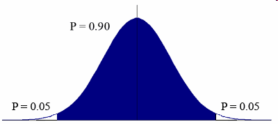
T-test computes the value of the T-statistics for our gene and than compare its value to this distribution under the null hypothesis. If the T-statistics is to extreme in comparison to the distribution of T-statistics when there is no difference, we can say that there is a difference in gene expression between cancer and normal group. The “extremity” of the T-statistics is actually its p-value.
In next section we will describe several basic methods, which help us to make statistically correct decision between null and alternative hypothesis.