E-learning in analysis of genomic and proteomic data 2. Data analysis 2.2. Analysis of high-density genomic data 2.2.1. DNA microarrays 2.2.1.5. Data pre-processing
Once the hybridized microarray slides were scanned and the resulting images analyzed by software for image analysis in order to get the intensity of each spot on array, we can start the analysis. First of all, it is necessary to carry out few pre-processing steps to enhance their quality. In following sections we will discuss several methods which is applied to make data more suitable for detailed analysis.
2.2.1.5.1. Raw data format
cDNA arrays
The raw data for each image were stored in a special text files with a specific format, dependent on the type of software used. For example data from GenePix software for image analysis have extension .gpr, data from Affymetrix extension .CEL etc. etc. All of these files are readable with any classic text or spreadsheet editor.
The information stored in the text file may vary according to the type of microarray experiment and the software used for image analysis; however, the most important information is common for all of them. Each row represents one spot on the microarray, columns represent different variables. For cDNA arrays these are usually:
- position of the spot on a microarray (either in pixels or the coordinates on the grid, most usually both)
- name and other identifications of a probe on the spot
- other information about the spot quality (size, shape, circularity, percentage of saturated pixels...)
- spot raw sample signal intensity (for one or two channels) and derived characteristics (mean, median, SD)
- background signal intensity around the spot (one or two channels) and derived characteristics (mean, median, SD)
- other derived characteristics (signal to noise ratio, log intensities, log ratio between two channels, …)
- flags – a summarized information about the spot quality in form of a qualitative variable represented usually as integer values. The value of the flag is assessed automatically by the image analysis algorithm according to settings or manually by the user.
affymetrix arrays
2.2.1.5.2. Quality control of raw data
cDNA arrays
As described above, the raw data received from a program for image analysis are usually arranged in a matrix, where rows are spots and each column correspond to different spot characteristic. For example there is information about spot intensity, like mean, median or intensity standard deviation for spot foreground and background, then there are some derived characteristics like signal to noise ratio or ratio of foreground and background intensity. Very important is the information about spot quality, like circularity or diameter of spot and a flag parameter summarizing the spot quality, assigning a spot a good, bad, not found or empty status. These labels can differ in different programs.
When we get the raw data file, first of all we have to check for the data quality. The available spot characteristics are very useful for such a control. The aim of this control is to adjust parameter indicating the spot quality. This process is sometimes called flagging.
Here we present different procedures of detection of unreliable spots and each analyst must decide individually with regard to the data which of these methods he will apply on his data.
First, the spots can be filtered according to their shape and size. This filter it is not applicable when fixed circle segmentation algorithm (all spots are selected to have equal diameter) of spot detection was used in image analysis program. The spot should be filtered out if it has too small diameter and the number of spot pixels is too low. When adaptive segmentation algorithm for spot detection was applied, the raw data contains also a parameter determining the spot circularity. If the circularity is highly disturbed, such a spot should be removed from the analysis. Sometimes we can find spot which is of so-called donut shape - the probes in the center did not hybridize. Such spots should be excluded too.
Another useful parameter is the percentage of saturated spot pixels. The program for image analysis should have assigned saturated spots with bad flag, however, it depends on settings and it is always necessarry to check the spot saturation ad-hoc.
Another important filtration is according to spot intensity. There are different of statistical measures that can be used for this filtering. We will mention two of them, namely signal to noise ratio - the proportion of foreground signal to standard deviation of background signal and foreground to background intensity ratio, where we expect (under the assumption of equal background intensity), that the ratio increases with the spot intensity.
Spots with too low intensity should be excluded. Each scanner has a different detection threshold. The more precise the scanner is the threshold can be lower. Keeping spots with too low intensities in analysis can lead to biased results, as the low intensity is very difficult to distinguish from overall background noise.
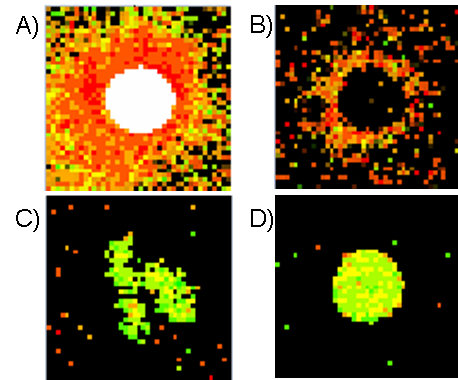
Figure: Different types of spots:
A) Saturated spot, B) Donut spot, C) Spot with non-circular shape, D) Good circular spot
affymetrix arrays
2.2.1.5.3. Transformations of raw data
When the data are filtered of bad spots, we should always check their distribution. Common way is drawing the histogram with reasonable number of intervals and visualize thus the data distribution. In microarray experiment the distribution of intensities is always positively skewed - this means the longer tail on right side towards the high intensities:

Numerically we can compare mean and median of the distribution. If the median is lower then the mean, the data are positively skewed and if median is higher, then the data are negatively skewed. Because many statistical tests assume data normality, the transformation is required. Additionally this transformation facilitate data visual inspection - the extremely high values would otherwise not allow to inspect lower and more frequent intensities (see the histogram on the left, where we cannot see the distribution of values from 0 to 100).
There are several transformations which can greatly reduce the skewness, but for the facility of the interpretation of the data, the log2 transformation is used in most cases. This transformation is defined as X->log2(X).
Sometimes the logarithm with different base are used (log10). Other transformation to mention is so called power transformation defined as X->Xa, where a>0.
The very important and special set of transformations connected to quality control that have to be applied to all the data is called the normalization of the data. It is very important and we describe it in the individual chapter.
2.2.1.5.4. Summarization
Summarization is an important last step after all the transformations have been performed. On the majority of microarrays each probe is spotted to multiple spots in order to minimize possible spatial errors and control the variability. The raw data thus contains multiple raws for each probe. For further analysis, only one value representing the probe is necessary. The aim of summarization is to get one representative measure for each probe.
cDNA arrays
The easiest way is to take the mean of all values, while controlling for standard deviation by excluding the most extreme values (trimmed mean) or median.
affymetrix arrays
The summarization techniques for affymetrix data slightly differ from those of cDNA arrays, because of the different design of arrays.