E-learning in analysis of genomic and proteomic data 2. Data analysis 2.2. Analysis of high-density genomic data 2.2.1. DNA microarrays 2.2.1.11. Pathway Analysis
2.2.1.11.3 Gene Set and Pathway Analysis Methods
We will now discuss how we can detect whether a given gene set (possibly obtained from one of the resources mentioned in the previous Section) is differentially expressed or not. Very many methods have been suggested for this problem over the last few years and instead of listing and discussing them one after the other, we will rather discuss the general characteristics that separate the various methods.
2.2.1.11.3.1 Self-contained vs Competitive Methods
We return to our Pima Indian microarray data set. As we saw in the last section we can identify 96 probe sets on this array that correspond the GO term ”inflammatory response”. The very first thing we can do is to check the outcome of the statistical test we already performed. For example we might count how many of the genes are significant at a 5% level, i.e. have an unadjusted p-value below 5%. It turns out to that 8 of the 96 genes are significant. The typical way of turning this result into p-value for the complete gene set is to ask: What is the probability to observe 8 significant out of 96 genes? As it turns out there two very different ways the term ”chance” can be interpreted in this question. These two options are to use either a self-contained or a competitive method, a distinction and terminology introduced by Goeman and Buhlmann [2007].
2.2.1.11.3.1.1 Self-contained testing
For a self-contained method we only use the values observed within the gene set of interest and ignore all other genes. The null hypothesis tested is
H0s = {”No gene in the gene set is differentially expressed”}
For a non-differentially expressed gene the chance to be significant at a 5% level is 5%, so we would expect 96 × 5% = 4.8 genes to be significant by chance. Obviously we observed more than that, but is the difference significant? To answer this question, we need to make the assumption that the genes are stochastically independent of each other, i.e. knowing the values for one gene, doesn’t give us any information about the other genes in the gene set (this is quite a strong assumption that will be discussed in more detail below). If this is the case, the number of significant genes in the set will follow a B(96, 0.05)-distribution, i.e. a binomial distribution with n = 96 and p = 0.05. We can then calculate a p-value as the probability of observing 8 or more significant genes under this distribution and obtain p = 10.8%, i.e. the result is not quite significant at a 5% level (it would need 10 out of 96 for that).
2.2.1.11.3.1.2 Competitive testing
In the competitive setting we compare the genes within the gene set to all other genes on the array, i.e. the null hypothesis is
H0s = {”The gene set is not more differentially expressed than other genes”}.
Comparing the formulation of the two null hypotheses it is obvious that this a fundamentally different approach. A competitive method will very much depend on the size of the microarray for example. If we had a very small array with just the 96 inflammatory genes on them for example, it would not be possible at all to conduct a competitive test. If the array is middle sized with thousand genes, the result will differ from a whole genome array with 40000 genes etc. In our situation we can conduct a competitive test by observing that out of 12639 genes on the array 1272 overall were significant (10.1%), which indicates that there are indeed substantial differences in gene expression between the two groups. If we randomly picked 96 genes from the array we would expect 96×10.1% ≈ 9.7 genes to be significant by chance, i.e. in this case the observed number is even less than we would expect under the null hypothesis. The data can be summarized in the 2 × 2 cross tabulation given in table 2.2.1.11.2.
Table 2.2.1.11.2: 2 × 2 cross table for the inflammatory gene set
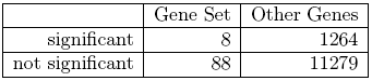
For this table we know want to test whether there is an association between the event ”Gene is significant” and ”Gene is in Gene Set”. The classical tests for this problem are the Chi-Square-Test or Fisher’s exact test. The former uses an asymptotic result to calculate p-values, which is not valid for tables with low expected frequencies. Fisher’s exact test uses the exact hypergeometric distribution, i.e. the probability of observing the given table given the marginal counts. In our situation the p-value obtained from Fisher’s test is p = 73.3 and thus far higher than the one observed with the self-contained test. Although the self-contained hypothesis seems to be the much more natural way of formulating our testing problem from a statistical point of view, competitive methods are widely used with Fisher’s exact test possibly even being the most popular method overall.
2.2.1.11.3.2 Methods not based on cut-offs
One problem with the methods discussed above is they rely on an arbitrary decision on which genes to call significant. Had we used a 10% p-value threshold for example our self-contained binomial test would have given us
a p-value of 2.2%, a much more convincing result. A stricter cut-off of 1% would yet again have produced a completely different result. By simply classifying genes a significant or not significant we loose a lot of potentially useful information. Knowing that the 88 non-significant genes in the gene set have a p-value very close to 5% is a very different situation from the one where those genes were far away from being significant.
2.2.1.11.3.2.1 The self contained Kolmogorov-Smirnov Test
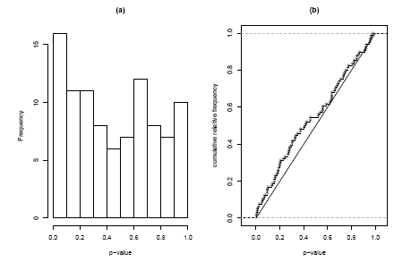
The solution to this problem is to use the full distribution of p-values in our test. In Figure 2.2.1.11.4(a) we see a histogram of the 96 p-values in the inflammation gene set. Under the self-contained null hypothesis, that no gene in the set is differentially expressed, we would expect the p-values to form a uniform distribution. What we see instead is indication of a peak at the left side. To decide whether this deviation of uniformity is significant we can use the Kolmogorov-Smirnov-test. This test is not based on the histogram, but on the cumulative distribution function. In Figure 2.2.1.11.4(b) we see the observed cumulative distribution function compared to the expected diagonal line. The Kolmogorov-Smirnov-Statistic is given by the maximum difference between these two curves and the corresponding p-value gives the probabilit of observing this difference or a larger on, if the p-values indeed were uniformly distributed. In our case we obtain p = 8.2%.
Figure 2.2.1.11.4: Histogram and cumulative distribution function of p-values corresponding to the self-contained Kolmogorov-Smirnov Test
2.2.1.11.3.2.2 The competitive Kolmogorov-Smirnov Test
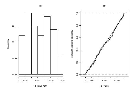
It is easy to find a competitive counterpart by replacing the p-values for our gene set with their ranks within all p-values; i.e. if a gene is the 835-smallest p-value on the array its rank will be 835. Under competitive null hypothesis now these ranks are expected to be uniformly distributed across the numbers from 1 to 12639 (the number of genes on the array). Again we can check this visually with a histogram or cumulative distribution plot (Figure 2.2.1.11.5), both of which do not show any striking evidence of non-uniformity. Again we can use the Kolmogorov-Smirnov statistic to test this formally and obtain a p-value of 85.1%, which confirms our visual impression. The two very different results of the self-contained and of the competitive test might seem confusing, but it must be kept in mind that these tests answer two very different question. The nearly significant p-value of the selfcontained test says ”there might be some differential expression in this gene set”, whereas the highly non-significant p-value of the competitive analysis says ”but the amount of differential expression is not larger than in general on the array”. These are non conflicting statements in a case where there seem to be many differentially expressed genes on the array. If these differential genes were equally distributed across the pathways present on the array we might find in the extreme case that a self-contained method declares all pathways to be significant, whereas a competitive method finds no significance at all.
Figure 2.2.1.11.5: Histogram and cumulative distribution function of p-values corresponding to the competitive Kolmogorov-Smirnov Test
2.2.1.11.3.3 Other analysis issues
The topics discussed so far might explain the most fundamental differences between different gene set analysis methods, but there are a number of other issues that need to be considered as well. We will discuss some of them in the following.
2.2.1.11.3.3.1 Direction of Test
Typically the p-values from a single-gene analysis stem from a two-sided test, i.e. we decide whether a gene is differentially expressed but do not differentiate between up or down-regulation. So when we use these p-values to perform a gene set analysis a gene set with the same amount of up and down-regulated genes can be as significant as another set that only contains up-regulated genes. It depends on the kind of gene set and the biological situation, whether changes in both directions within a gene set are of interest or not. If not the afore mentioned method can be easily adapted to detect up or down-regulated gene sets by using p-values from the corresponding one-sided test.
3.3.2 Dependence between genes
As we mentioned in Section 2.2.1.11.3.1.1 we so far assumed that the genes within our gene set were stochastically independent under the null hypothesis. This is quite unlikely because particularly genes with a similar function or within the same pathway tend to have correlated gene expression profiles. To see how this affects the methods we discussed let us consider the extreme case that all genes in the gene set will always have identical expression. In that case we only need to analyse that one gene and its p-value will present the complete set. However, both the binomial test and Fisher’s exact test will either have a p-value very close to zero (if the p-value of the gene is significicant and thus all p-values in the set are significant) or close to 1 (if the gene is not significant), i.e. these test will completely misrepresent the true evidence. Of course the example of completely correlated genes is unrealistic but milder correlations will still bias the results.
3.3.3 Resampling methods
Many approaches do not use an asymptotic or theoretical distribution to calculate p-values, but a resampling approach. By either permuting the arrays or the genes new versions of the data set can be calculated for which the statistic of interest is re-calculated. All possible permutations or a large random set of such permutations are generated, which gives us a distribution for the statistic which is then being used to calculate a p-value. Fisher’s exact test for example is a test that is based on gene resampling. Resampling genes is directly connected to a competitive hypothesis, whereas array resampling corresponds to a self-contained hypothesis. The problem of correlations between genes can be solved by using array resampling. If we used this approach instead of the binomial distribution for testing the self-contained hypothesis the resampled data sets would keep this correlation structure and thus give a valid p-value. Resampling genes however doesn’t help in this situation, unless we assume that all genes on the array are equally correlated to eachother.
3.3.4 Multiple Testing
So far we discussed the analysis of one gene set (in our example given by a single GO term) only. However, typically this kind of analysis is conducted on many gene sets simultaneously, e.g. all GO terms that belong to the biological process node or all human pathways available from KEGG. Just as when testing single genes we thus have to address the multiple testing problem that 1 in 20 gene sets will be declared significant by chance, if we apply the usual 5% threshold to the p-value for the gene set. With gene set analysis we face an additional problem though: even if we assume that individual genes are stochastically independent, the same will not be true for gene sets which often overlap. The problem is particularly bad when dealing with GO terms as these are hierarchically arranged, i.e. certain terms will define gene sets that are subsets of others. This issue is too complex to discuss it in detail in this introductory text, but we should mention that one method can be applied without any problem in this situation: The traditional Bonferroni method to control the family wise error rate makes no assumption about independence of tests, so it will work in any gene set situation, although it can be very conservative.
3.3.5 Replicated Genes
On many microarrays a gene is represented by more than one probe, and often the number of replicates per gene is different from gene to gene. Obviously this can affect the analysis in a negative way, e.g. if one particular gene of a set is differentially expressed but has multiple copies on the array it will make the complete gene set look more changed than it actually is. The best solution for this problem is to combine the values of the replicates to one number prior to gene set analysis. In the case of Affymetrix arrays using Custom CDF annotation files [Dai et al., 2005] for preprocessing partly solves the problem as the re-annotation of the arrays is designed to combine all probes representing the same gene. For other cases averaging across replicates is a widely used solution. Note that such averaging should be done for the original normalised gene expression values and not for data summaries like p-values (an average of p-values will no longer be uniformly distributed under the null hypothesis, i.e. it will not be valid p-value itself).